7. Diffusion Models

This chapter discusses main ideas of diffusion models behind many modern generative tools. These models are particularly powerful in applications like text-to-image and text-to-video generation.

1. Variational Autoencoders (VAEs)

1.1 The Basics

Recall the following concept from our Chapter 1:

• : The distribution of , typically unknown and complex.

• : The distribution of , often assumed to have standard Gaussian prior whose dimension is smaller than .

• : The encoder, proxy for .

• : The decoder, proxy for .

• The objective function for VAEs is the maximization of the Evidence Lower Bound (ELBO)

• Loss Function: We approximate the first term by Monte-Carlo simulation:

where is the -th sample in the training set, and is sampled from . The distribution is parameterized by .

Then the training loss of VAE is given by

(1)

You may verify that the KL divergence has an analytic expression.

After training a VAE, generating new data can be performed by sampling directly from the latent space and then running it through the decoder.

1.2 Hierarchical Variational Autoencoders (HVAEs)

A Hierarchical Variational Autoencoder (HVAE) extends the concept of VAEs by introducing multiple layers of latent variables.

General HVAE has hierarchical levels and each latent is allowed to condition on all previous latents. We instead focus on a special case called Markovian HVAE (MHVAE). In a MHVAE, the generative process is a Markov chain, i.e., decoding each only conditions on . See below for a MHVAE.

Figure: A Markovian HVAE (image source)

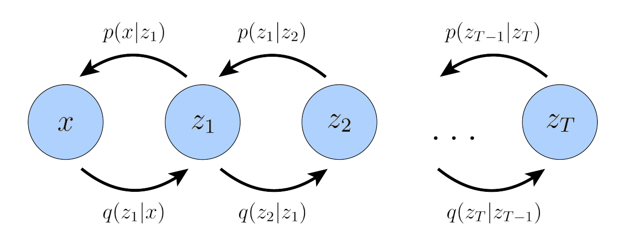
The joint distribution and the posterior of a MHVAE is given by

and

The ELBO of such model can be written as

2. Denoising Diffusion Probabilisitc Model (DDPM)

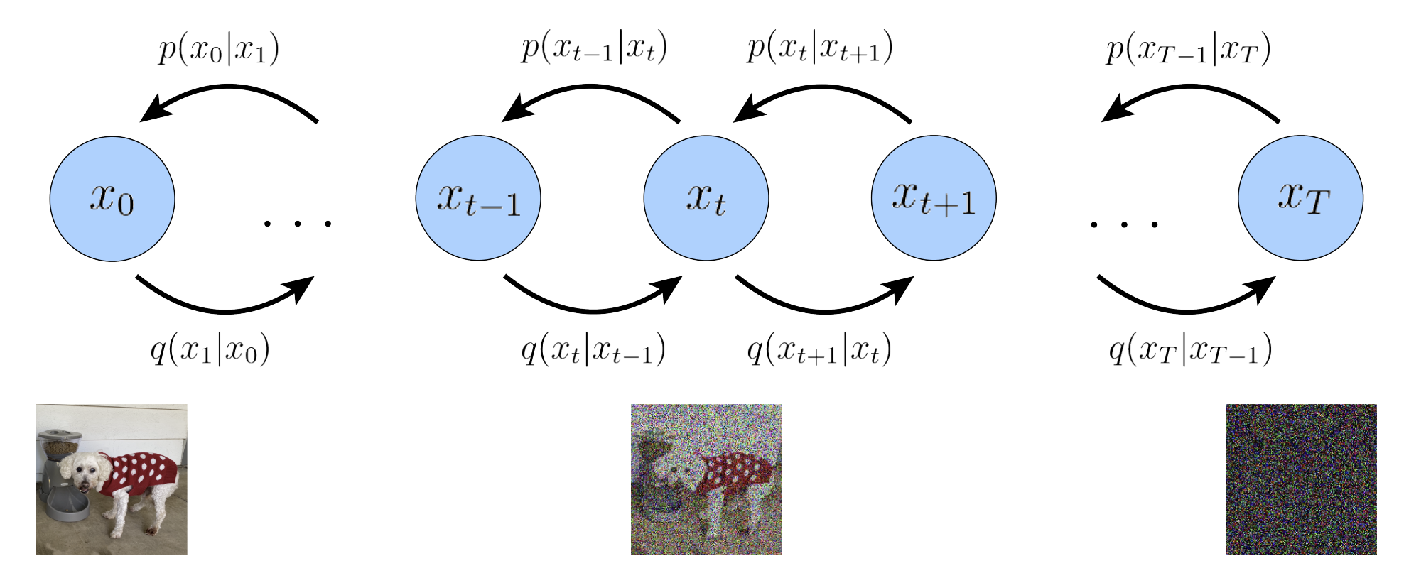
A Denoising Diffusion Probabilisitc Model (DDPM) is a MHVAE with below three restrictions:

• Restriction 1: The latent dimention is equal to the data dimention

Basically a DDPM has a sequence of states , where is the original image, are the latent variables with the same dimension as .

The DDPM posterior can now be rewritten as

• Restriction 2: The latent encoder at each timestep is pre-defined as a linear Gaussian model

Here we parameterize the encoder as

or

where is a (potentially learnable) coefficient that can vary per time . This form of coefficients are chosen for being variance-preserving.

• Restriction 3: The parameters of the Gaussian latent encoders are set to vary over time such that the distribution of the latent at the final timestep is a standard Gaussian

is set to evolve such that . In DDPM paper the noise schedule is set for and linearly increasing from to , .

Now the joint distribution for a DDPM can be rewritten as

where

Note our encoders are no longer parameterized by , while our decoders (denoising transitions) are learnable to approach the transition distributions .

The full process of the encoders (adding noises) and decoders (denoising) is shown below.

Figure: A visual representation of DDPM (image source)

2.1 ELBO of DDPM

There are two ways to understand the ELBO of DDPM.

The first way is to write

Reconstruction Term

The reconstruction term is derived from the expectation over the conditional distribution . This term predicts the log probability of the original data sample given the first-step latent . This is similar to the decoder phase in a standard VAE, where the model learns to regenerate the original input from its latent representation, enhancing the model’s ability to capture and reconstruct the input data accurately.

Prior Matching Term

The prior matching term involves the KL divergence between the final latent distribution and the Gaussian prior. This term is minimized when the distribution of the final latent variable closely matches the Gaussian prior .

Consistency Term

The consistency term checks for the consistency of the latent space transformation across all intermediate steps. It ensures that the forward transformation to a noisier image matches the reverse transformation from a cleaner image, making the distribution at consistent.

Under this derivation, all terms of the ELBO are computed as expectations, and can therefore be approximated using Monte Carlo estimates. However, optimizing the ELBO using the terms we just derived might be suboptimal: because the consistency term is computed as an expectation over two random variables for every timestep, the variance of its Monte Carlo estimate could potentially be higher than a term that is estimated using only one random variable per timestep. As it is computed by summing up consistency terms, the final estimated value of the ELBO may have high variance for large values.

The second way tries to compute expectation over only one random variable at a time:

(2)

Reconstruction Term (same as above)

The reconstruction term is the same as in the first derivation.

Prior Matching Term

This term involves the KL divergence between the final latent distribution and a Gaussian prior. Under assumptions that the final latent distribution approximates a Gaussian, this term often evaluates to zero. This simplification reflects the model’s adherence to the prior distribution without requiring trainable parameters.

Denoising Matching (Consistency) Term

The consistency term measures the fidelity of the denoising transitions It ensures that the model’s denoising capability, from a noisier to a cleaner state, matches the theoretical ground-truth denoising transition defined by . This term is minimized when the model’s predicted denoising steps closely align with these ground-truth transitions.

This second interpretation of the ELBO offers a framework for understanding and implementing each component with reduced computational complexity and increased intuitive clarity. By focusing on one random variable at a time, we achieve lower variance in estimates, leading to more stable and reliable model training outcomes in variational inference frameworks like VAEs.

2.2 ELBO Continued: computational details

For ELBO derived in the (2), we need the explicit form of and for sampling.

We present the result here:

or equivalently

where and .

where

(3)

and

2.3 Two equivalent ways of modeling

2.3.1 First Way of Modeling

From the ELBO (2) we know that we have to compute the KL divergence term. is what we can set for training, and from 2.3 we know is Gaussian, so for convenience we formulate as a Gaussian, with the same variance as and a learnable mean:

where is a neural network parametrized by .

Now we have

(4)

To match the form of mean in (3)

we set

where is another neural network (still parameterized by ) that predicts the clean image from the noisy image and time .

Now the KL divergence (4) can be further simplified to

Note that for our reconstruction term in (2) we can derive that

Therefore, the training of the neural network based on the ELBO we derived boils down to the simple loss function below:

2.3.2 Second Way of Modeling

Note that we set our neural network () for predicting the image. We can actually learn to predict the noise. To see that, from we can obtain and put it in , and then get

So similarly we can design our mean estimator as

And the new loss function would be given by

The training and inference process below is what you would see in the DDPM paper. We elaborate on them below.

Training a Denoising Diffusion Probabilistic Model

• Repeat the following steps until convergence.

• For every image ( is the batch size) in a batch for training: sample a random time stamp .

• Draw a sample

• Draw a sample by

• Take gradient descent step on

Inference on a Denoising Diffusion Probabilistic Model

• Sample an .

• Repeat the following for .

• Calculate .

• Update according to

Sample Code: Training a DDPM in Practice

Install some packages:

pip install git+https://github.com/huggingface/diffusers.git#egg=diffusers[training]
pip install accelerate
pip install datasets

Set up configurations:

from dataclasses import dataclass

@dataclass
class TrainingConfig:
    image_size = 128  # the generated image resolution
    train_batch_size = 16
    num_epochs = 50
    gradient_accumulation_steps = 1
    learning_rate = 1e-4
    lr_warmup_steps = 500
    save_image_epochs = 10
    save_model_epochs = 30
    mixed_precision = 'fp16'  # `no` for float32, `fp16` for automatic mixed precision
    output_dir = 'ddpm-butterflies-128'  
    seed = 0

config = TrainingConfig()

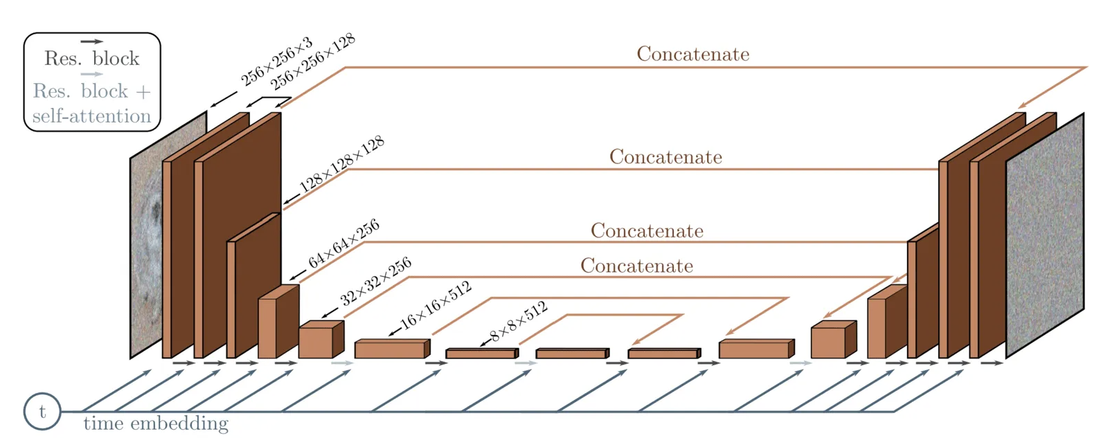
The denoising neural network is often a U-Net in practice. The input would be an RGB image and the timestep , and the output would also be an RGB image.

Figure: A U-Net architecture used in DDPM (image source)

from diffusers import UNet2DModel

model = UNet2DModel(
    sample_size=config.image_size,  # the target image resolution
    in_channels=3,  # the number of input channels, 3 for RGB images
    out_channels=3,  # the number of output channels
    layers_per_block=2,  # how many ResNet layers to use per UNet block
    block_out_channels=(128, 128, 256, 256, 512, 512),  # the number of output channes for each UNet block
    down_block_types=( 
        "DownBlock2D",  # a regular ResNet downsampling block
        "DownBlock2D", 
        "DownBlock2D", 
        "DownBlock2D", 
        "AttnDownBlock2D",  # a ResNet downsampling block with spatial self-attention
        "DownBlock2D",
    ), 
    up_block_types=(
        "UpBlock2D",  # a regular ResNet upsampling block
        "AttnUpBlock2D",  # a ResNet upsampling block with spatial self-attention
        "UpBlock2D", 
        "UpBlock2D", 
        "UpBlock2D", 
        "UpBlock2D"  
      ),
)

This UNet2DModel consists of the following blocks

Input Convolution

• Conv2d(3, 128, kernel_size=(3, 3), stride=(1, 1), padding=(1, 1))

  • Maps 3-channel images to 128 feature channels.

Time Embedding

• Timesteps(): Generates embeddings for different time steps.

• TimestepEmbedding

  • Linear(in_features=128, out_features=512, bias=True): Projects time embeddings to a higher dimension.

  • SiLU(): Activation function for adding non-linearity.

  • Linear(in_features=512, out_features=512, bias=True): Further processing of the time embeddings.

Downsampling Blocks

• Sequence of DownBlock2D modules, each containing:

  • Residual Blocks (ResnetBlock2D)

    • GroupNorm(32, width, eps=1e-05, affine=True): Normalizes the features within each group.

    • Conv2d(width, width, kernel_size=(3, 3), padding=(1, 1)): Maintains feature width.

    • Linear(in_features=512, out_features=width, bias=True): Projects time embeddings.

    • SiLU(): Adds non-linearity between convolutional layers.

    • Dropout(p=0.0, inplace=False): Optional dropout (inactive here) for regularization.

  • Downsampling

    • Conv2d(width, width, kernel_size=(3, 3), stride=(2, 2), padding=(1, 1)): Reduces spatial dimensions.

Mid Block

• UNetMidBlock2D

  • Attention

    • GroupNorm(32, 512, eps=1e-05, affine=True) and linear layers for queries, keys, and values.

    • Attention: Captures global dependencies across features.

  • Residual Blocks (ResnetBlock2D)

    • Structured similarly to those in the downsampling stages, focused on bottleneck features.

Upsampling Blocks

• Sequence of UpBlock2D modules, each containing:

  • Residual Blocks (ResnetBlock2D)

    • Structured similarly to downsampling but integrates lower-level features.

  • Upsampling

    • Conv2d(width, width, kernel_size=(3, 3), stride=(1, 1), padding=(1, 1)): Increases spatial dimensions.

The dataset we use here is Butterflies dataset. It consists of 1000 images for butterflies from different species. We need to resize them for training.

from datasets import load_dataset
import torch
from torchvision import transforms

config.dataset = "huggan/smithsonian_butterflies_subset"
dataset = load_dataset(config.dataset, split="train")

preprocess = transforms.Compose(
    [
        transforms.Resize((config.image_size, config.image_size)),
        transforms.RandomHorizontalFlip(),
        transforms.ToTensor(),
        transforms.Normalize([0.5], [0.5]),
    ]
)

def transform(examples):
    images = [preprocess(image.convert("RGB")) for image in examples["image"]]
    return {"images": images}

dataset.set_transform(transform)

train_dataloader = torch.utils.data.DataLoader(dataset, batch_size=config.train_batch_size, shuffle=True)

To inspect what the images look like, you can use the code below

import matplotlib.pyplot as plt
fig, axs = plt.subplots(1, 4, figsize=(16, 4))
for i, image in enumerate(dataset[:4]["images"]):
    axs[i].imshow(image.permute(1, 2, 0).numpy() / 2 + 0.5)
    axs[i].set_axis_off()
fig.show()

And you will see figures like this

Figure: Some examples of resized images from Butterflies

The scheduler function here can basically do two things according to the specific diffusion process: 1. add noise to the image for training. 2. remove the noise based on the model output for inference. We use DDPMScheduler for noise scheduler, which means that we will do the above two things according to the linear schduler from to by default, with .

from diffusers import DDPMScheduler

noise_scheduler = DDPMScheduler(num_train_timesteps=1000)

Then we can start training with the code below

from diffusers.optimization import get_cosine_schedule_with_warmup
from accelerate import Accelerator
from tqdm.auto import tqdm
import torch
import torch.nn.functional as F
optimizer = torch.optim.AdamW(model.parameters(), lr=config.learning_rate)
lr_scheduler = get_cosine_schedule_with_warmup(
    optimizer=optimizer,
    num_warmup_steps=config.lr_warmup_steps,
    num_training_steps=(len(train_dataloader) * config.num_epochs),
)

def train_loop(config, model, noise_scheduler, optimizer, train_dataloader, lr_scheduler):
    # Initialize accelerator
    accelerator = Accelerator(
        mixed_precision=config.mixed_precision,
        gradient_accumulation_steps=config.gradient_accumulation_steps
    )
    
    # Prepare everything
    model, optimizer, train_dataloader, lr_scheduler = accelerator.prepare(
        model, optimizer, train_dataloader, lr_scheduler
    )
    
    global_step = 0

    # train the model
    for epoch in range(config.num_epochs):
        progress_bar = tqdm(total=len(train_dataloader), disable=not accelerator.is_local_main_process)
        progress_bar.set_description(f"Epoch {epoch}")

        for step, batch in enumerate(train_dataloader):
            clean_images = batch['images']
            # Sample noise to add to the images
            noise = torch.randn(clean_images.shape).to(clean_images.device)
            bs = clean_images.shape[0]

            # Sample a random timestep for each image
            timesteps = torch.randint(0, noise_scheduler.num_train_timesteps, (bs,), device=clean_images.device).long()

            # Add noise to the clean images according to the noise magnitude at each timestep
            noisy_images = noise_scheduler.add_noise(clean_images, noise, timesteps)
            
            with accelerator.accumulate(model):
                # Predict the noise residual
                noise_pred = model(noisy_images, timesteps)["sample"]
                loss = F.mse_loss(noise_pred, noise)
                accelerator.backward(loss)

                optimizer.step()
                lr_scheduler.step()
                optimizer.zero_grad()
            
            progress_bar.update(1)
            global_step += 1

        # Save the model at the end of training
        if accelerator.is_main_process and epoch == config.num_epochs - 1:
            model.save_pretrained(config.output_dir)

# Directly call the train loop with the arguments
train_loop(config, model, noise_scheduler, optimizer, train_dataloader, lr_scheduler)

Inference with the above trained DDPM

To use a trained DDPM like above, we need the utility function download_and_unzip from utils.py to load files for the trained model shared through Google Drive.

from utils import download_and_unzip
trained_ddpm_id = '1h675AhteNxXd752FCqqcRMu0TSkuupCY'
output_dir= # e.g., "models/"
checkpoint = download_and_unzip(trained_ddpm_id, output_dir) 

import os
from diffusers import UNet2DModel
from diffusers import DDPMScheduler

model = UNet2DModel.from_pretrained(checkpoint)
scheduler = DDPMScheduler(num_train_timesteps=1000)

Then we can do sampling in this way. It would show the final output together with the intermideate samples.

import torch
import PIL.Image
from IPython.display import display
import numpy as np
import tqdm

def display_sample(sample, i):
    # Convert tensor to image for visualization
    image_processed = sample.cpu().permute(0, 2, 3, 1)
    image_processed = (image_processed + 1.0) * 127.5
    image_processed = image_processed.numpy().astype(np.uint8)

    # Create PIL Image and display it with step info
    image_pil = PIL.Image.fromarray(image_processed[0])
    display(f"Image at step {i}")
    display(image_pil)

model.to("cuda")
scheduler.alphas_cumprod = scheduler.alphas_cumprod.to("cuda")
image_size = 128
# Initialize the noise sample
torch.manual_seed(0)
noisy_sample = torch.randn(
    1, 3, image_size, image_size  # Ensure this matches your model's expected input
).to("cuda")
sample = noisy_sample

# Inference loop through the timesteps
for i, t in enumerate(tqdm.tqdm(scheduler.timesteps)):
    # Predict the noise residual
    with torch.no_grad():
        residual = model(sample, torch.tensor([t]).to(sample.device)).sample  # Ensure your model call is correct

    # Compute denoised image and update sample
    sample = scheduler.step(residual, torch.tensor([t]).to(sample.device), sample).prev_sample

    # Display image at specified timestep
    if (i + 1) % 50 == 0:
        display_sample(sample, i + 1)

The final output will look like this

Figure: An example of the output from the trained DDPM

Inference with others’ pretrained DDPM

To illustrate inference, we also use another pretrained DDPM google/ddpm-celebahq-25. The code below shows how to load this model and do the denoising process for one image. The sampling may take a few minutes for only one image.

from diffusers import DDPMPipeline, UNet2DModel, DDPMScheduler
import PIL.Image
import numpy as np
import torch
import tqdm

# load the pretrained DDPM
image_pipe = DDPMPipeline.from_pretrained("google/ddpm-celebahq-256")
image_pipe.to("cuda")
repo_id = "google/ddpm-church-256"
model = UNet2DModel.from_pretrained(repo_id)
scheduler = DDPMScheduler.from_config(repo_id)

# display the image for intermediate steps
def display_sample(sample, i):
    image_processed = sample.cpu().permute(0, 2, 3, 1)
    image_processed = (image_processed + 1.0) * 127.5
    image_processed = image_processed.numpy().astype(np.uint8)

    image_pil = PIL.Image.fromarray(image_processed[0])
    display(f"Image at step {i}")
    display(image_pil)
model.to("cuda")

# sample the initial noise
torch.manual_seed(0)
noisy_sample = torch.randn(
    1, model.config.in_channels, model.config.sample_size, model.config.sample_size
)
noisy_sample = noisy_sample.to("cuda")
sample = noisy_sample

# do inference
for i, t in enumerate(tqdm.tqdm(scheduler.timesteps)):
  # predict noise residual
  with torch.no_grad():
      residual = model(sample, t).sample

  # compute denoised image and set x_t -> x_t-1
  sample = scheduler.step(residual, t, sample).prev_sample

  # optionally look at image
  if (i + 1) % 50 == 0:
      display_sample(sample, i + 1)

3. Score-Matching Langevin Dynamics (SMLD)

3.1 Langevin Dynamics

Langevin dynamics is a stochastic process described by a differential equation that models the evolution of a system under the influence of both deterministic and random forces. The continuous-time Langevin dynamics is given by the following stochastic differential equation (SDE):

where is the target probability distribution, and is a standard Wiener process (Brownian motion).

A key property of this SDE is that its stationary distribution coincides with . In other words, as , the distribution of converges to . This convergence property makes Langevin dynamics a powerful tool for sampling from complex probability distributions.

To generate samples from , one can simulate the Langevin dynamics for a sufficiently long time. The resulting trajectory will explore the state space according to the target distribution, with the gradient term guiding the process towards high-probability regions and the stochastic term ensuring exploration of the entire space.

In practice, simulating the continuous-time process is often infeasible, so a discrete-time approximation is used. The discrete Langevin dynamics for sampling from is an iterative procedure for :

where is the step size that users can control, and is typically initialized as white noise.

This discrete approximation converges to samples from the target distribution as and . In practice, a small but finite step size is used. Metropolis-adjusted Langevin algorithm is often used to correct approximation biases.

3.2 Score Matching Techniques

Since we have no access to , we need approximation of . In this section we introduce two of such approximation.

We define as the neural network parameterized by that predicts the score function.

Explicit Score-Matching

Given dataset , consider the classical kernel density estimation (KDE) with

where is the bandwidth for the kernel function . is then an approximation to the unknown true data distribution .

The explicit score matching loss is then given by

Once we train the network , we can do sampling with

The problem with explicit score matching is that KDE is poor estimation of the true distribution, especially when the number of samples is limited or the samples are high-dimensional.

Denoising Score Matching

It can be shown that the following loss, also known as Denoising Score Matching (DSM),

(5)

satisfies

where is a term that does not depend on . Refer to this paper that connects ESM and DSM.

Now the loss function (5) is highly interpretable: the score function is trained to take the noisy image and predict the noise .

The training step is as follows: given a training dataset , train a network with the goal

There are some empirical problems found with above score matching:

• The score function is ill-defined when lies on a low-dimensional manifold in a high-dimensional space.

• The estimated score function trained will not be accurate in low density regions.

• Langevin dynamics sampling may not mix, even if it is performed using the ground truth scores.

To address the problems in such vanilla score matching, an empirical solution is proposed: Add multiple levels of Gaussian noise to the data. Specifically, choose a positive sequence of noise levels , , and define a sequence of progressively perturbed data distributions

such that and .

Then, a neural network is trained using score matching to learn the score function for all noise levels simultaneously:

where is a positive weighting function that conditions on noise level , and often chosen as based on empirical findings.

Empirically, the annealed Langevin dynamics sampling is applied as a sampling procedure: samples are produced by running Langevin dynamics for each in sequence:

For each noise level , steps of Langevin MCMC are run sequentially for each :

where is the step size, and is standard normal.

The sampling start with and set for As and for all , becomes an exact sample from

This is analogous to the sampling procedure performed in DDPM, where a randomly initialized data vector is iteratively refined over decreasing noise levels.

4. Stochastic Differential Equations (SDE)

Diffusion models implement a discrete-time formulation with a finite number of noise scales. A natural question arises: how can we extend this framework to continuous time, effectively allowing for an infinite number of noise scales?

This extension not only provides a more flexible modeling approach but also establishes a deeper connection between diffusion models and continuous-time stochastic processes. To understand this connection, we need to introduce the concept of Stochastic Differential Equations (SDEs).

4.1 A Gentle Introduction of SDE

4.1.1 From Discrete to Continuous: Introducing Brownian Motion

Consider a discrete-time diffusion process and then extend it to continuous time. We start by discretizing the continuous time interval into equal steps. Let be the index of these discrete time steps, so that , where is the time step size. In discrete time, we assume a general diffusion process:

where is a drift function, and represents Gaussian noise.

To move to continuous time, we introduce Brownian motion (also known as a Wiener process), denoted as . Brownian motion has the following key properties:

1. almost surely

2. For , the increment is normally distributed with mean 0 and variance

3. The increments are independent for non-overlapping time intervals

4.1.2 Formulating SDE

Using Brownian motion, we can now write our continuous-time diffusion process as an SDE:

Here:

• is the drift term, representing the deterministic part of the process

• is the diffusion term, representing the random fluctuations

• is a time-dependent diffusion coefficient

This SDE can be interpreted as the limit of our discrete process as :

Note that doesn’t exist in the classical sense, but it can be understood as “white noise” in a distributional sense.

4.1.3 Forward and Reverse SDEs

In the context of diffusion models, we are particularly interested in two types of SDEs:

1. Forward SDE: This describes the process of gradually adding noise to the data:

   

2. Reverse SDE: As an important result, this describes the reverse process of removing noise to generate samples:

   

   where is the probability density of at time , and is a Brownian motion in reversed time.

The reverse SDE is crucial for generative modeling, as it allows us to start from pure noise and gradually refine it into a sample from the data distribution. The term is the score function, which needs to be estimated to solve the reverse SDE. Next we will present the result of discretizing reverse SDE as a sampling method for DDPM and SMLD respectively.

4.2 SDE for DDPM

The discrete-time DDPM iteration is given by

(6)

for This forward sampling equation can be written as an SDE via

(7)

We can say the DDPM iteration (6) solves the SDE (7), but it may not be the best solver.

The corresponding reverse-time SDE is then given by

Discretization of the reverse SDE above gives us a way to sample with DDPM:

4.3 SDE for SMLD

The perturbed data distribution used in SMLD can be derived by induction from the following Markov chain

assuming , , and .

The forward SDE of SMLD can then be written as

The reverse-time SDE for this would be

Similar to DDPM case we have the following discretization for sampling:

5. Diffusion Model in Practice: Stable Diffusion

5.1 Overview

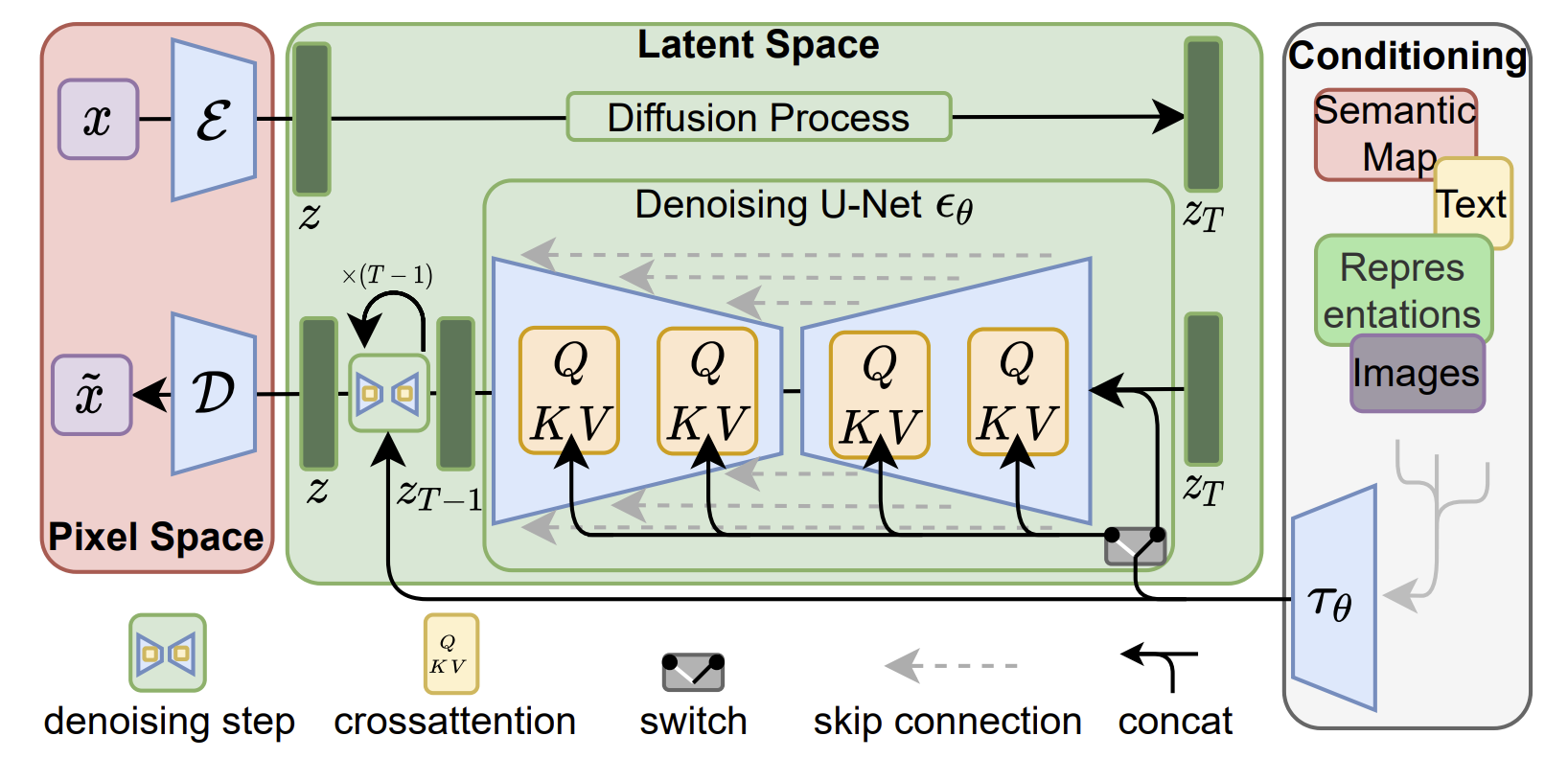
Stable Diffusion (SD) is a popular text-to-image model based on diffusion. Stable Diffusion series before SD 3 is essencially a Latent Diffusion Model (LDM) with three components: an autoencoder, a U-Net based conditional denoisng network, and a text encoder.

The autoencodng model learns a low-dimentional latent space that is perceptually equivalent to the image space. It was empirically shown that the denosing U-Net works on the latent space much more efficiently than denoising directly on the high-dimensional image space. The text encoder accepts text input and guides the diffusion process.

5.2 Details of Architecture

5.2.1 The Autoencoder

Given an image in RGB space, the encoder encodes into a latent representation , and the decoder reconstructs the image from the latent, giving , where . Trained similarly as VAE.

5.2.2 The (Conditional) Denoising U-Net

The Denoising U-Net in SD is similar to that in DDPM , a time-conditional U-Net, except that now it works on the low-dimensional latent space. Since the forward process is fixed, can be efficiently obtained from during training, and samples from can be decoded to image space with a single pass through .

In SD, the U-Net is turned to a conditional image generator with the augmentation of cross-attention. It is effective for learning attention-based models of various input modalities.

5.2.3 Conditioning Mechanisms

In principle, diffusion models can model conditional distributions of the form . This can be implemented with a conditional denoising neural network where inputs (such as text or image) would guide the diffusion process.

To pre-process from various modalities (such as language prompts), a domain specific encoder is introduced to project to an intermediate representation . It is then mapped to the intermediate layers of the U-Net via a cross-attention layer implementing , with

Here, denotes a (flattened) intermediate representation of the U-Net that models . and are learnable projection matrices. This is shown below.

Figure: Overview of LDM (image source)

Based on image-conditioning pairs, the conditional LDM is learned via

where both and are jointly optimized. This conditioning mechanism is flexible as can be parameterized with domain-specific experts, e.g. (unmasked) transformers when are text prompts.

We list some common cases of conditional generation.

• For text-to-image generation, the is often a transformer architecture.

• For layout-to-image generation, we discretize the spatial locations of the bounding boxes and encode each box as a -tuple, treated as the above . Here, denotes the (discrete) top-left and the bottom-right position. Class information is represented by . The is also often implemented as a transformer.

Figure: Examples of Layout-to-Image Generation with LDM (image source)

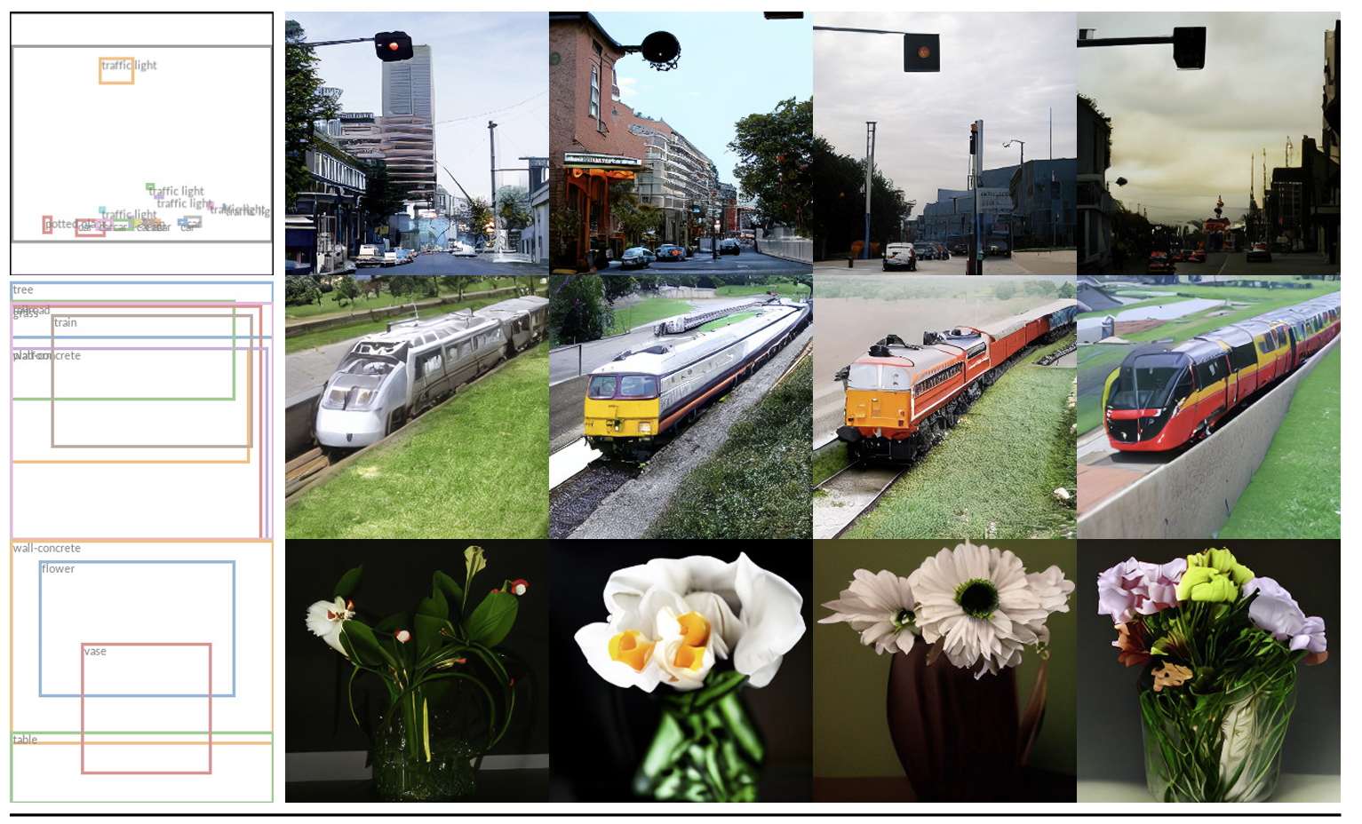
• For the class-conditional generation, is a single learnable embedding layer with a dimension (e.g., 512), mapping a class to a vector .

References

• Tutorial on Diffusion Models for Imaging and Vision

• Understanding Diffusion Models: A Unified Perspective

• Auto-Encoding Variational Bayes

• Denoising Diffusion Probabilistic Models

• Variational Diffusion Models

• Score-Based Generative Modeling through Stochastic Differential Equations

• Reverse-Time Diffusion Equation Models

• Generative Modeling by Estimating Gradients of the Data Distribution

• High-Resolution Image Synthesis with Latent Diffusion Models